
Precision-Recall Trade-off and ROC/AUC (optional)
We discuss the precision-recall trade-off at different decision probability thresholds, and introduce another useful evaluation metric, ROC/AUC, which is especially helpful for imbalanced datasets.
This page continues from Model Evaluation and Selection: it uses the same Titanic split and the same three trees, with tree_clf3 already trained on X_train.
Decision Probability and Threshold
In classification, the final prediction for a data point is actually a probability score. For example, for one person in the Titanic dataset, a prediction looks like [0.38, 0.62]: the predicted probability that this person died (0) is 0.38, and that they survived (1) is 0.62. The default decision threshold is 0.5, so this person is predicted to be 1 (survived). But if we raised the threshold to 0.7, the same person would be predicted to be 0 (died).
predict_proba returns both probabilities for every test passenger:
plt.style.use('ggplot')

# we have 179 predictions
X_test.shape  # (179, 3)

# for each prediction there are two probabilities, one per label: 0 means died, 1 means survived
y_pred_proba = tree_clf3.predict_proba(X_test)
print(y_pred_proba[0])  # [0.384 0.616] -> 0.38 died, 0.62 survived
y_pred_proba.shape      # (179, 2)
Putting the probabilities next to the predictions shows the 0.5 threshold at work — every passenger with P(survived) of 0.5 or more is predicted to survive:
results = pd.DataFrame({
    'P(died)': y_pred_proba[:, 0],
    'P(survived)': y_pred_proba[:, 1],
    'prediction': y_pred,  # from tree_clf3.predict(X_test)
    'actual': y_test.values,
})
results.head()
P(died) P(survived) prediction actual
0 0.384 0.616 1 1
1 0.597 0.403 0 0
2 0.529 0.471 0 0
3 0.384 0.616 1 1
4 0.597 0.403 0 1The Precision-Recall Trade-off
Changing the decision threshold changes precision and recall. Raising it makes the model more cautious about predicting "survived": the passengers it does predict to survive are more likely to be right (higher precision), but it misses more of the real survivors (lower recall). Lowering it does the opposite. On this test set:
| Threshold | Precision | Recall |
|---|---|---|
| 0.3 | 0.590 | 0.838 |
| 0.5 (default) | 0.722 | 0.527 |
| 0.7 | 0.758 | 0.338 |
Increasing precision usually decreases recall and vice versa — the precision-recall trade-off.
Why? Both share the numerator TP, but raising the threshold changes their denominators in different ways. Here are the counts behind the table — 74 passengers in the test set actually survived:
| Threshold | Predicted survived (TP + FP) | TP | FP | FN | Precision = TP / (TP + FP) | Recall = TP / (TP + FN) |
|---|---|---|---|---|---|---|
| 0.3 | 105 | 62 | 43 | 12 | 62 / 105 = 0.590 | 62 / 74 = 0.838 |
| 0.5 | 54 | 39 | 15 | 35 | 39 / 54 = 0.722 | 39 / 74 = 0.527 |
| 0.7 | 33 | 25 | 8 | 49 | 25 / 33 = 0.758 | 25 / 74 = 0.338 |
- Recall goes down. Its denominator TP + FN is the number of actual survivors, 74, whatever the threshold. A higher threshold predicts fewer passengers to survive, so some real survivors move from TP to FN. TP shrinks over a fixed denominator, so recall can only fall.
- Precision usually goes up. Its denominator TP + FP is everyone the model predicts to survive. A higher threshold drops the passengers the model was least sure about, and those are mostly FP. From 0.3 to 0.5, FP falls by 28 (43 → 15) while TP falls by only 23 (62 → 39): the group predicted to survive loses its mistakes faster than its correct predictions, so a larger share of what is left is correct.
It is only usually: if a step drops more TP than FP, precision falls as well. You can see it in the chart below, where precision drops above a threshold of about 0.75 — the model's most confident predictions are not always its most accurate. Which one to favor depends on the context, as in Uneven Costs of Two Types of Prediction Errors.
precision_recall_curve computes precision and recall at every useful threshold at once:
# the score of the positive class (survived) is the 2nd column
y_scores = y_pred_proba[:, 1]

# precision and recall at different thresholds; y_test holds the true labels
# https://scikit-learn.org/stable/modules/generated/sklearn.metrics.precision_recall_curve.html
from sklearn.metrics import precision_recall_curve
precisions, recalls, thresholds = precision_recall_curve(y_test, y_scores)

print(precisions.shape, recalls.shape, thresholds.shape)  # (13,) (13,) (12,)
There is one more precision and recall value than there are thresholds: the last precision is 1 and the last recall is 0, and they have no threshold. So we drop them with [:-1] when plotting against the thresholds:
from sklearn.metrics import PrecisionRecallDisplay

fig, ax = plt.subplots(1, 2, figsize=(15, 5))

ax[0].plot(thresholds, precisions[:-1], label='Precision')
ax[0].plot(thresholds, recalls[:-1], label='Recall')
ax[0].set_title('Precision and Recall at Different Thresholds')
ax[0].set_xlabel('Threshold')
ax[0].legend()

PrecisionRecallDisplay.from_predictions(y_test, y_scores, ax=ax[1], name='Tree 3')
ax[1].set_title('Precision-Recall Curve')
ax[1].legend()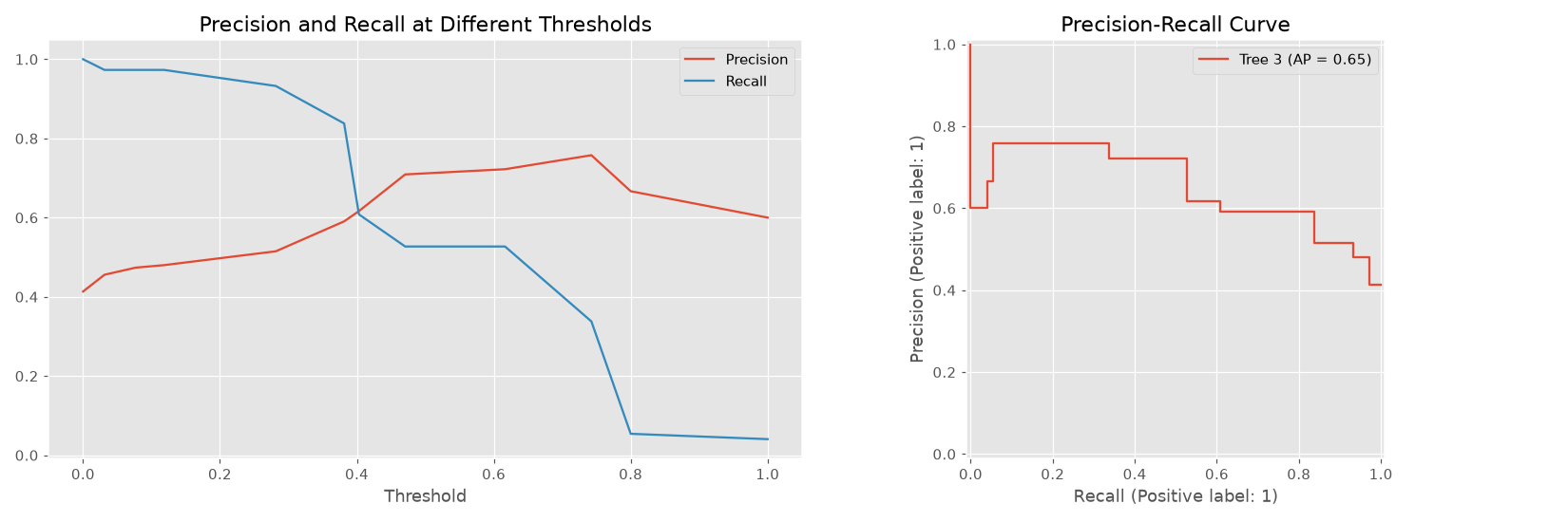
The left chart is the trade-off: as the threshold rises, recall falls and precision (mostly) rises. The right chart plots the same pairs against each other. Its legend shows average precision (AP), a single number summarizing the whole curve — higher is better.
ROC Curve and AUC
The Receiver Operating Characteristic (ROC) curve is another way to evaluate a classifier across all thresholds. It plots two rates, both read from the confusion matrix:
- True Positive Rate (TPR) = TP / (TP + FN) — this is just recall: of the real positives, how many are caught.
- False Positive Rate (FPR) = FP / (FP + TN) — of the real negatives, how many are wrongly predicted positive.
Lowering the threshold catches more survivors (TPR up) but also predicts more of the passengers who died to survive (FPR up). The ROC curve traces that trade from threshold 1 (bottom-left: nobody is predicted to survive) to threshold 0 (top-right: everybody is). See the scikit-learn ROC example for more details.
from sklearn.metrics import roc_curve
fpr, tpr, thresholds = roc_curve(y_test, y_scores)

fig, ax = plt.subplots()

ax.plot(fpr, tpr, label='Tree 3')
ax.plot([0, 1], [0, 1], linestyle='--', color='gray', label='Random guessing')
ax.set_title('ROC Curve')
ax.set_xlabel('False Positive Rate')
ax.set_ylabel('True Positive Rate (Recall)')
ax.legend()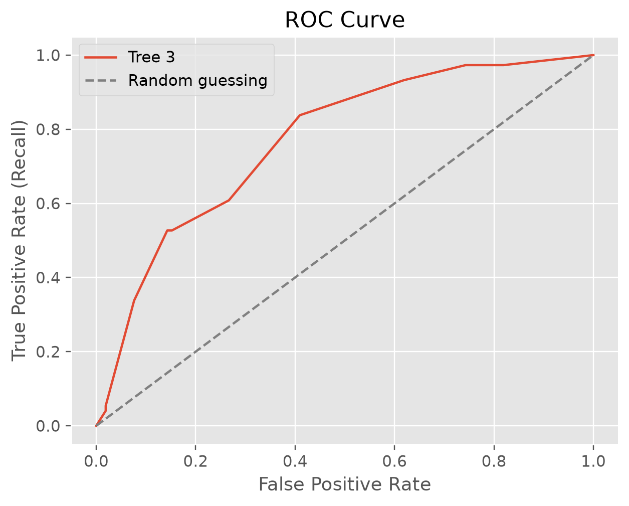
The dashed diagonal is a model that guesses at random. The further the curve bows toward the top-left corner — catching every positive with no false alarms — the better the model.
AUC (Area Under the ROC Curve) turns the curve into one number between 0 and 1:
- 0.5 — no better than random guessing (the area under the diagonal)
- 1.0 — a perfect model
AUC also has a plain-language meaning: pick one passenger who survived and one who died at random; AUC is the probability that the model gives the survivor the higher survival score.
from sklearn.metrics import roc_auc_score
roc_auc_score(y_test, y_scores)  # 0.770
Comparing Models with ROC/AUC
AUC is useful for comparing models, because it does not depend on any one threshold. Let's train the other two trees and compare all three:
# train the other two trees on the same training data
tree_clf1.fit(X_train, y_train)
tree_clf2.fit(X_train, y_train)

# the score of the positive class (survived) for each tree
y_scores_1 = tree_clf1.predict_proba(X_test)[:, 1]
y_scores_2 = tree_clf2.predict_proba(X_test)[:, 1]

fpr_1, tpr_1, thresholds_1 = roc_curve(y_test, y_scores_1)
fpr_2, tpr_2, thresholds_2 = roc_curve(y_test, y_scores_2)

print(f'AUC score for tree 1 is {roc_auc_score(y_test, y_scores_1):.3f}')
print(f'AUC score for tree 2 is {roc_auc_score(y_test, y_scores_2):.3f}')
print(f'AUC score for tree 3 is {roc_auc_score(y_test, y_scores):.3f}')

fig, ax = plt.subplots()

ax.plot(fpr_1, tpr_1, label='Tree 1')
ax.plot(fpr_2, tpr_2, label='Tree 2')
ax.plot(fpr, tpr, label='Tree 3')
ax.plot([0, 1], [0, 1], linestyle='--', color='gray', label='Random guessing')
ax.set_title('ROC Curve')
ax.set_xlabel('False Positive Rate')
ax.set_ylabel('True Positive Rate (Recall)')
ax.legend()
AUC score for tree 1 is 0.682
AUC score for tree 2 is 0.751
AUC score for tree 3 is 0.770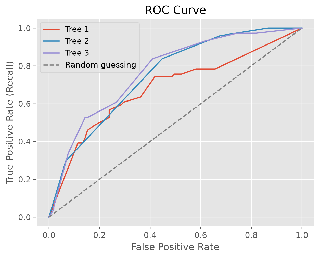
Tree 3 is slightly better than tree 2: it has the higher AUC, and its curve comes closer to the top-left corner. Tree 1 — the tree with no depth limit — is clearly the weakest, the same verdict cross validation gave in Model Evaluation and Selection.
The trees in Model Evaluation and Selection are created with random_state=42, so you should get these same numbers.
Imbalanced Data
For classification problems with very imbalanced data — such as COVID-19 test results, where far more people test negative than positive — the default threshold can result in poor model performance. A model that predicts "negative" for everyone scores a high accuracy while catching no one. ROC/AUC is often a better metric than accuracy for imbalanced data.
"For those classification problems that have a severe class imbalance, the default threshold can result in poor performance. As such, a simple and straightforward approach to improving the performance of a classifier that predicts probabilities on an imbalanced classification problem is to tune the threshold used to map probabilities to class labels."
See a nice tutorial on this topic: A Gentle Introduction to Threshold-Moving for Imbalanced Classification.
Model Evaluation and Selection
NOTE: In order to keep this demonstration code simple, we only choose three numerical features to train the model to avoid the tedious categorical feature…
Model Evaluation In-Class Exercise
In the Heuristic Challenge you wrote rules by hand, and a good rule landed in the mid 0.70s on accuracy. Today you hand the same data to a decision tree and…