Gradient Descent

Gradient Descent (GD) is a generic optimization algorithm that can be applied to a wide range of problems.

The basic idea of GD is to iteratively tweak model parameters to minimize the cost function (error function or loss function) such as MSE we learned before.

The basic idea of GD is as follows:

"Suppose you are lost in the mountains in a dense fog, and you can only feel the slope of the ground below your feet. A good strategy to get to the bottom of the valley quickly is to go downhill in the direction of the steepest slope" (source: https://bit.ly/3tVy6rQ)

GD measures the local gradient of the cost function with regard to the parameter vector $\mathbf\theta$ and goes in the direction of descending gradient.

Once the gradient is zero, the minimum is reached.

The basic steps are:

random initialization: fill $\mathbf\theta$ with random values
take one small step (measured by the learning rate eta $\eta$ ) at a time trying to decrease the cost function (MSE)
repeat till reaching the minimum (algorithm convergence) or approach arbitrarily close to the minimum

As shown in the figure below:

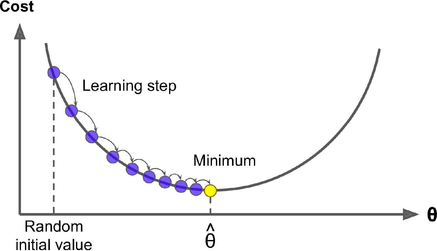
Images Credits: https://www.oreilly.com/library/view/hands-on-machine-learning/9781492032632/

Learning Rate $\eta$ (eta)

If we set the learning rate too small, it may take a long time to converge:

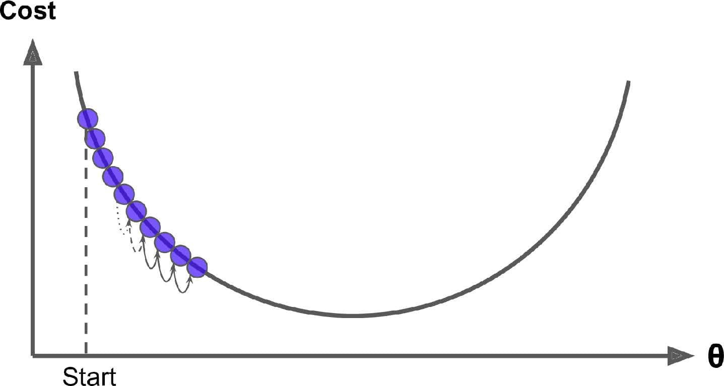
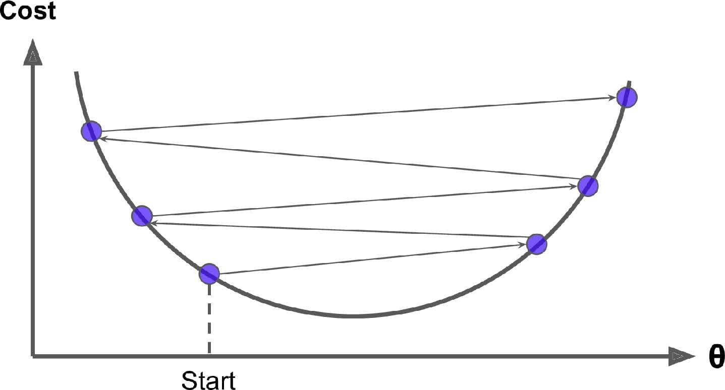
If we set the learning rate too large, the algorithm may jump around and even diverge:

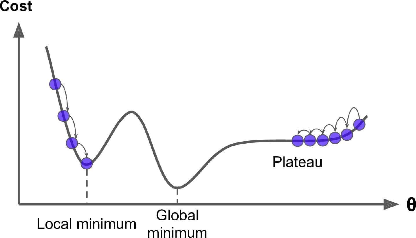
When the cost function is not convex (not like a bowl, with holes, ridges, plateaus, etc.), the algorithm may find only the local minimum or take a long time to cross the plateaus - we do a few random initialization hoping to land to the place that can lead us to the global minimum quickly.

NOTE: The cost function MSE is a convex function, which guarantees a global minimum.

We will cover three types of GD:

Batch Gradient Descent (BGD)
Stochastic Gradient Descent (SGD)
Mini-batch Gradient Descent

Batch/Full Gradient Descent (BGD)

Some basic knowledge of Calculus is needed:

Derivatives of a function with one variable using various rules (Power, Product, Quotient): https://www.youtube.com/watch?v=QqF3i1pnyzU
Derivatives of multivariable functions: https://www.khanacademy.org/math/multivariable-calculus/multivariable-derivatives
Non-Differentiable functions https://en.wikipedia.org/wiki/Differentiable_function

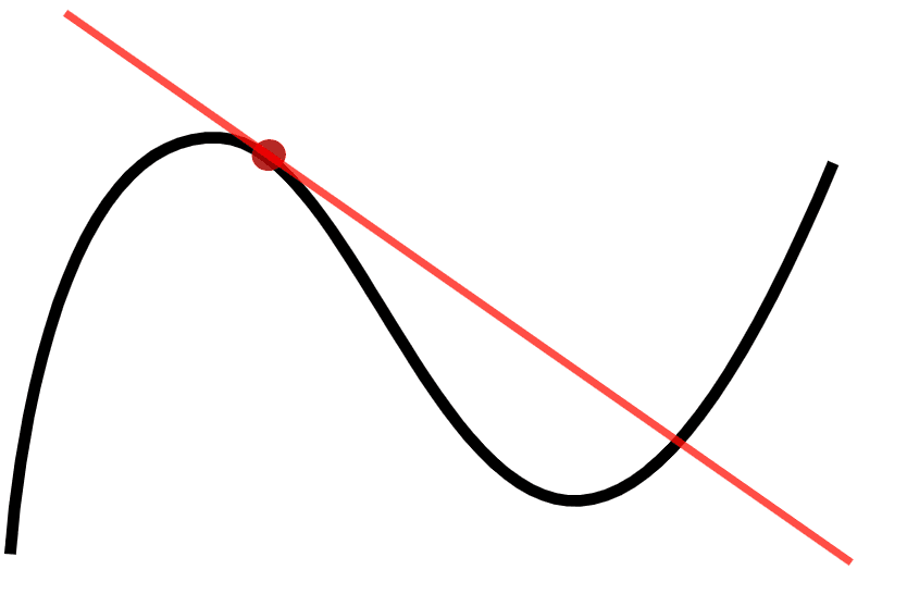
An Example (https://en.wikipedia.org/wiki/Derivative):

black curve is the graph of a function
red line is the a tangent line to the functions
the slope of the tangent line is the derivative of the function at the marked point

BGD Steps for Linear Regression

Calculate partial derivative for ONE Theta $\theta_j$

Recall the cost function for linear regression is MSE:
$MSE(\mathbf{\theta}) = \frac{1}{m} \sum_{i=1}^m (\mathbf{\theta}^\top\mathbf{x}^{(i)} - y^{(i)})^2$
The partial derivative of the cost function with regard to ONE model parameter $\theta_j$ is:
$\frac{\partial}{\partial \theta_j}MSE(\mathbf{\theta})= \frac{2}{m} \sum_{i=1}^m (\mathbf{\theta}^ \top \mathbf{x}^{(i)} - y^{(i)}) x_j^{(i)}$
This means how much the cost function is going to change if you just change $\theta_j$ a little bit - "what's the slope of the mountain under my feet if I face $\theta_j$ direction".

NOTE: here you need to use ALL m rows to calculate the partial derivative given $\theta_j$ affect every row of the dataset.
Calculate partial derivatives for ALL Theta $\mathbf\theta$ to get Gradient Vector $\nabla_{\mathbf{\theta}}$ (Nubla)

ALL partial derivatives for the cost function for all $\mathbf{\theta}$ can be calculated as the Gradient Vector of the cost function $\nabla_{\mathbf{\theta}}$ (Nubla):
$\nabla_{\mathbf{\theta}}MSE(\mathbf{\theta})=\begin{pmatrix} \frac{\partial}{\partial\theta_0}MSE(\mathbf{\theta})\\ \frac{\partial}{\partial\theta_1}MSE(\mathbf{\theta})\\ \vdots \\ \frac{\partial}{\partial\theta_n}MSE(\mathbf{\theta}) \end{pmatrix}= \frac{2}{m}\mathbf{X}^\top(\mathbf{X}\vec{\theta} - \mathbf{y})$
IMPORTANT NOTE: $\nabla_{\mathbf{\theta}}MSE(\mathbf{\theta})$ is calculated in EACH STEP of the Gradient Descent using the FULL training dataset.

Therefore, Batch GD (maybe Full GD is a better name) could be very slow on very large dataset!!!
Update all Theta for the next step with learning rate Eta

Now, we can calculate the GD step:
$\mathbf{\theta}^{\text{(next step)}} = \mathbf{\theta} - \eta \nabla_{\mathbf{\theta}}MSE(\mathbf{\theta})$
Here eta $\eta$ is the learning rate, which decides the size of the step. A common default value for the learning rate eta is 0.1 or 0.01. eta is often tuned via grid search from 0.1 to 10^-6.
Repeat 1-3 with updated $\mathbf{\theta}$ and full training dataset

Next, we will compare linear regression and BGD and see they will generate the same optimal result:

# let's generate some linear looking data
# the ideal model apparently is y = 5 + 3x

import numpy as np
import matplotlib.pyplot as plt
plt.style.use('seaborn')

np.random.seed(42) # fix the random seed so that each run generates the same set of random numbers
X = 2 * np.random.rand(100, 1)  # generate 100 random numbers between 0 and 2 with shape (100, 1)
y = 5 + 3 * X + np.random.randn(100, 1)  # generate 100 random numbers from a normal distribution

fig, ax = plt.subplots()
ax.plot(X, y, ".")
ax.plot(X, 5+3*X)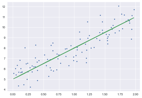

# Linear Regression via Scikit-Learn
import numpy as np

np.random.seed(42) # fix the random seed so that each run generates the same set of random numbers
X = 2 * np.random.rand(100, 1)  # generate 100 random numbers between 0 and 2 with shape (100, 1)
y = 5 + 3 * X + np.random.randn(100, 1)  # generate 100 random numbers from a normal distribution

from sklearn.linear_model import LinearRegression
lin_reg = LinearRegression()
lin_reg.fit(X, y) 
print(lin_reg.intercept_, lin_reg.coef_)

Output:
[5.21509616] [[2.77011339]]

try BGD:

# Batch Gradient Descent from Scratch
import numpy as np

np.random.seed(42) # fix the random seed so that each run generates the same set of random numbers
X = 2 * np.random.rand(100, 1)  # generate 100 random numbers between 0 and 2 with shape (100, 1)
y = 5 + 3 * X + np.random.randn(100, 1)  # generate 100 random numbers from a normal distribution

X_with_bias = np.c_[np.ones((100,)), X] # add bias term coefficient x0 = 1 for each instance

eta = 0.1  # the learning rate
n_iterations = 1000  # how many "steps" we take 
m = len(X_with_bias)  # number of training data

theta = np.random.randn(2, 1) # random initialization of theta with shape (2, 1)
print(f'Initial theta is \n{theta}')

for iteration in range(n_iterations):  # go over the whole training set 1000 times
    gradients = 2/m * X_with_bias.T.dot(X_with_bias.dot(theta) - y)  # this is gradient vector nubla
    theta = theta - eta * gradients  # update theta

# after 1000 steps we get exactly the same result of normal equation
print(f'theta after {n_iterations} is \n{theta}')

Output:

Initial theta is 
[[-0.26465683]
 [ 2.72016917]]
theta after 1000 is 
[[5.21509616]
 [2.77011339]]

Effects of Learning Rate and Total Iterations

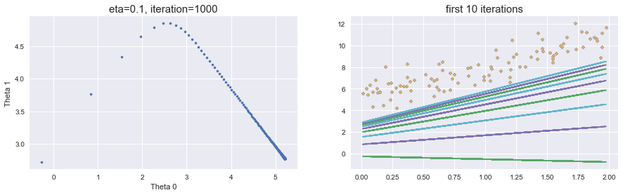
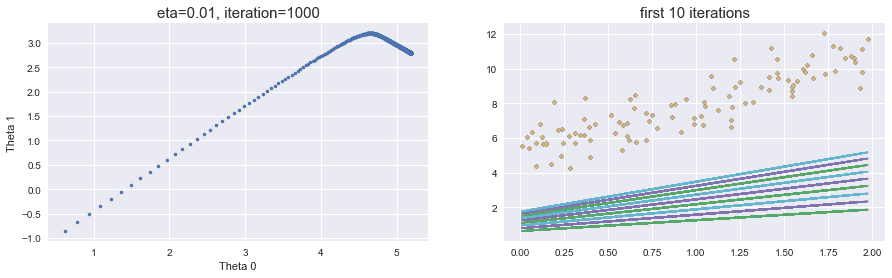
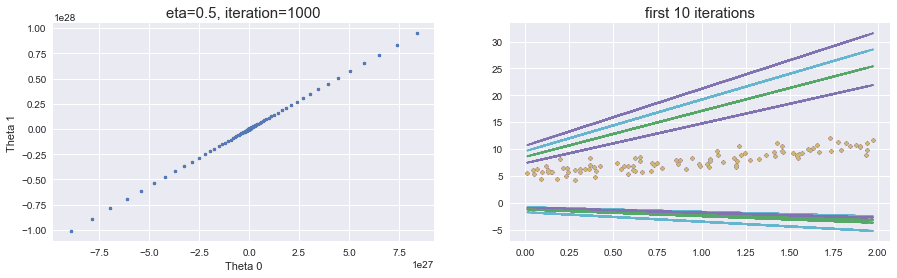
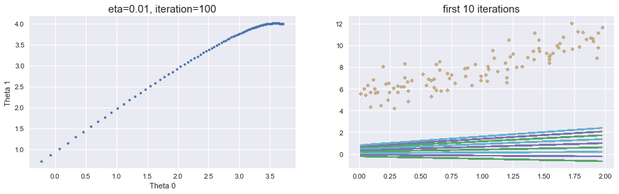
Next, we show how different values of learning rates and different number of iterations can affect BGD. The value of learning rate eta $\eta$ can be fine tuned via grid search.

BGD converged to the optimal model

take a smaller step, same 1000 steps - not converged to the optimal yet

take large steps, same 1000 steps - not even converging!!

small step and stop too early to get to the minimum

Stopping via Tolerance $\epsilon$ (epsilon)

How to set the value of iterations to avoid the situation like stopped too early?

One solution is:

Set a very large iteration number
Set a tiny threshold called tolerance $\epsilon$ (epsilon).
Stop when the norm of the gradients is smaller than the tolerance.

If $\mathbf{u} \in \mathbf{R}^n$ , the Norm of $\mathbf{u}$ is denoted as $\Vert \mathbf{u} \Vert$ , which is defined as the length or magnitude of the vector and is calculated using $\Vert \mathbf{u} \Vert = \sqrt{u_1^2+u_2^2+\ldots + u_n^2}$ .

Tolerance is often specified using scientific notation: tol=1e-3

# you should know scientific notation https://www.mathsisfun.com/numbers/scientific-notation.html
# 1.e-04 is 0.0001
np.format_float_scientific(0.0001)

Stochastic Gradient Descent (SGD)

BGD vs. SGD

Batch Gradient Descent (BGD) uses the FULL training set to calculate the gradients at each step. SGD instead only randomly pick ONE instance to compute the gradients in each step.

Think about BGD is like “look at all directions and choose sort of the average of all descents from all directions to take the next step” vs. SGD just randomly choose one direction and take the step.

BGD gently decreases to the optimal if the learning rate and iteration number are appropriate, while SGD tends to bounce up and down and decreases on average.
BGD can become very slow when the training set is large while SGD is much faster

NOTE: number of iterations in BGD is called number of epochs in SGD - same meaning

In summary, the final parameter values of SGD may not be optimal but often good enough given the huge gain on training speed.

# Stachastic Gradient Descent with fixed learning rate
# SGD is able to get close to the optimal
import numpy as np

n_epochs = 50 # this was called n_iterations for BGD
eta = 0.1  # the learning rate

m = len(X_with_bias) # number of training data, 100 in this case
theta = np.random.randn(2, 1) # random initialization 

for epoch in range(n_epochs): # go over the whole training set 100 times
    for i in range(m): # note: range(stop) begins at 0 and ends at stop – 1
        random_index = np.random.randint(m)  # get a random number between 0 and m
        xi = X_with_bias[random_index:random_index+1]  # randomly choose ONE instance x_i from the training dataset
        yi = y[random_index:random_index+1]  # choose the corresponding y_i
        gradients = 2 * xi.T.dot(xi.dot(theta) - yi)  # calculate the gradient for one instance
        theta = theta - eta * gradients  # update the gradient

print(theta)

Annealing (Learning Schedule)

When getting to the minimum, in order to keep SGD from jumping too much, one solution is to gradually reduce the value of the learning rate, which is called annealing (slowly cooling down).

The intuition is to take smaller and smaller steps when getting close to the optimal.

Learning schedule refers to the function that controls the learning rate at each step.

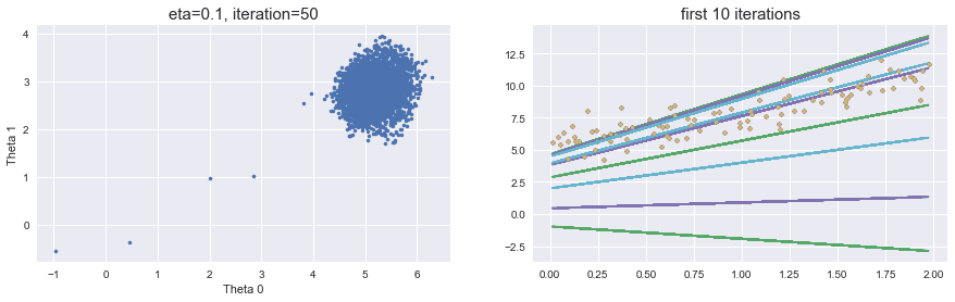
SGD with fixed learning rate (eta=0.1) - lots of bouncing around

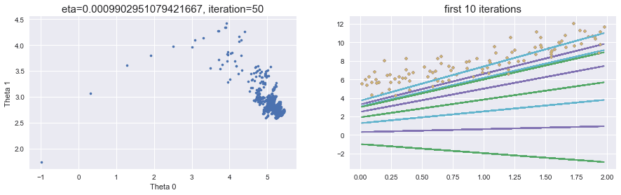
SGD with a learning schedule - compared with the example above, the steps became smaller and smaller and more concentrated:

Mini-batch Gradient Descent

SGD uses only ONE random instance to calculate gradients at each step, while BGD uses the FULL training set. Mini-BGD uses a random subset of the training data to calculate gradients at each step - less erratic than SGD but much faster than BGD.

SGD via Sklearn

Next, we use the housing dataset to train a SGD regressor and compare with the Linear regressor (RMSE: 81324) we trained in the previous lecture.

Example 1: this model's RMSE is a huge number - horrible result - the model was not even converging!

Lessons learned:

simple regressor without tuning often lead to horrible results
feature scaling is very important for SGD

# SGD without feature scaling
# stop after 1000 epochs or when loss drops below 0.001/1e-3
# eta0 is the initial eta with default invscaling learning schedule

import pandas as pd

df = pd.read_csv("housing.csv")

# for simplicity let's only choose population, median_income, housing_median_age to train the model 
# split train and test sets
X_housing = df[['population', 'median_income','housing_median_age']]
y_housing = df['median_house_value']

# split train/test
from sklearn.model_selection import train_test_split
X_train_housing, X_test_housing, y_train_housing, y_test_housing = train_test_split(X_housing, y_housing, test_size=0.2, random_state=42)

# simple sgd regressor
# this model's RMSE is a huge number - horrible result - the model was not even converging
# feature scaling and parameter tuning needed!!
from sklearn.linear_model import SGDRegressor
sgd_reg_housing = SGDRegressor(max_iter=1000, tol=1e-3, eta0=0.1)

sgd_reg_housing.fit(X_train_housing, y_train_housing)  # train the model

y_pred_housing = sgd_reg_housing.predict(X_test_housing)  # prediction

from sklearn.metrics import mean_squared_error

sgd_mse_housing = mean_squared_error(y_test_housing, y_pred_housing) 
sgd_rmse_housing = np.sqrt(sgd_mse_housing)
print(sgd_rmse_housing)

Example 2: SGD with feature scaling and parameter tuning vis grid search - much better results!

import numpy as np
import pandas as pd

df = pd.read_csv("housing.csv")

# for simplicity let's only choose population, median_income, housing_median_age to train the model 
# split train and test sets
X_housing = df[['population', 'median_income','housing_median_age']]
y_housing = df['median_house_value']

# split train/test
from sklearn.model_selection import train_test_split
X_train_housing, X_test_housing, y_train_housing, y_test_housing = train_test_split(X_housing, y_housing, test_size=0.2, random_state=42)

# sgd regression pipeline with feature scaling and grid search
# RMSE is about 81395 - better than without tuning
from sklearn.preprocessing import StandardScaler
from sklearn.pipeline import Pipeline
from sklearn.linear_model import SGDRegressor

sgd_reg_pipeline = Pipeline(
    steps=[
        ('scaler', StandardScaler()),
        ('sgd_reg', SGDRegressor()),
    ]
)

from sklearn.model_selection import GridSearchCV

param_grid = [
    {
        'sgd_reg__max_iter':[100000, 1000000],  # if number is too small, you will get a warning
        'sgd_reg__tol':[1e-10, 1e-3],
        'sgd_reg__eta0':[0.001, 0.01]
    }
]

# sgd regression grid search
sgd_grid_search = GridSearchCV(sgd_reg_pipeline, param_grid, cv=10)

sgd_grid_search.fit(X_train_housing, y_train_housing)

# sgd regression - best model
sgd_best = sgd_grid_search.best_estimator_
print('The best model is: \n', sgd_best)

# sgd regression - make prediction
y_pred_best_housing = sgd_best.predict(X_test_housing)

# calculate RMSE
from sklearn.metrics import mean_squared_error

sgd_rmse = np.sqrt(mean_squared_error(y_test_housing, y_pred_best_housing))
print(f'rmse: {sgd_rmse}')

On this page