Ensemble Learning

**Wisdom of the crowd：**the collective opinion of a group of individuals is often better than a single expert's answer.
Ensemble Learning: the prediction of a group of predictors often out-performs the best individual predictor.

Three Types of Ensemble Learning

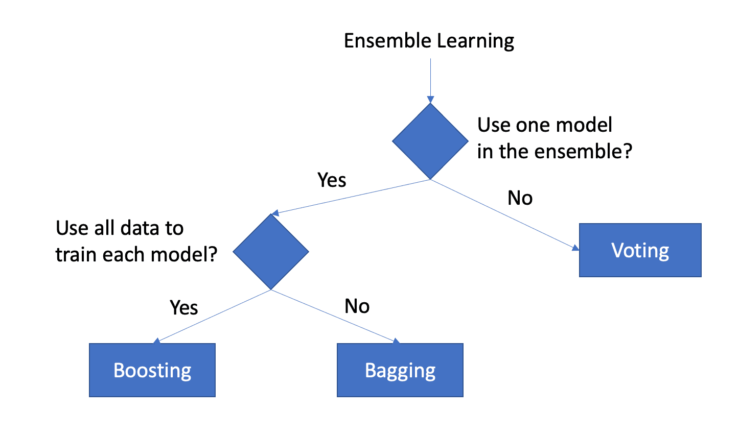
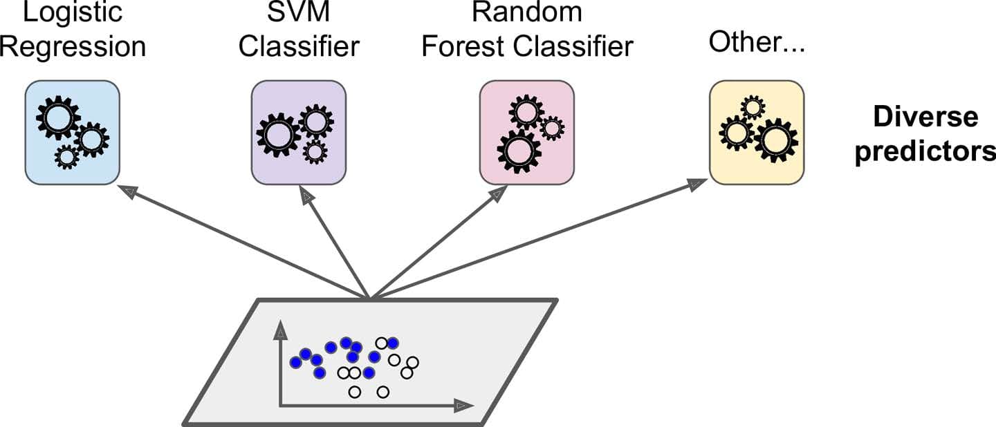
Screen Shot 2022-05-04 at 8.46.56 PM.png

Voting: ensemble of different models trained on all data

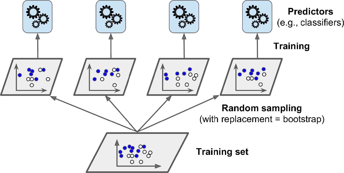
Bagging (Bootstrap Aggregation**):** ensemble of one model trained on different subsets of the dataset in parallel, such as Random Forest

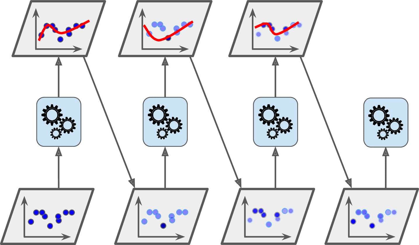
Boosting: Ensemble of one model trained on the same dataset sequentially, each trying to correct its predecessor, such as AdaBoost, Gradient Boosting, XGBoost

The general idea of boosting is to train predictors sequentially using all data, each trying to correct its predecessor.

Images Credits

The Bias/Variance Trade-off

Prediction Error = Bias + Variance + Noise

The prediction errors of a model (aka generalization error) can be expressed as the sum of three different errors:

Bias: measures the degree of the wrong assumptions of the model, such as assuming the data is linear when it's actually quadratic. A high-bias model means the assumption is very wrong, which often leads to the under-fitting problem.

High Bias (very wrong assumption) --> Under-fitting
Errors due to Variance: measures the degree of the sensitivity of the model to small variances in the training data. A high-variance model means that a little change in the data would greatly affect the model, which is essentially the overfitting problem.

High Variance (very sensitive to little changes in the data) --> Overfitting
Errors due to Noise: these errors are due to the noises of the data and are hard to reduce High Noise —> Collecting more data

Bias/Variance Trade-off: when we try to lower the bias using a more sophisticated model, such as a decision tree with many branches and deep depth, we also increase the variance of the model (it's easier for a complex decision tree to overfit the data).

Voting: reduce the bias by aggregating different models (different assumptions)
Bagging and boosting: reduce the variance by trained on different subset or updated dataset

Voting

Classification: once each model gives its prediction, we can use hard or soft voting to get the final prediction result.
Regression: the average of all predictions is used to be the final prediction.

Hard vs. Soft Voting

hard voting (majority voting): simply count the votes and predict using the majority of the votes
soft voting: if the classifiers are able to estimate the class probabilities, soft voting predicts the class label based on the highest class probability averaged over all individual classifiers

Hard voting predictions:

Classifier 1 predicts class A
Classifier 2 predicts class B
Classifier 3 predicts class B

2/3 classifiers predict class B, so class B is the ensemble decision.

Soft voting predictions:

Classifier 1 predicts class A with probability 0.9
Classifier 2 predicts class B with probability 0.55 (A 0.45)
Classifier 3 predicts class B with probability 0.55 (A 0.45)

The average probability of being class A across all classifiers is (0.9 + 0.45 + 0.45) / 3 = 0.6 (which is > 0.5 decision boundary) Therefore, class A is the ensemble decision.

We create some data to illustrate hard and soft voting:

# load packages
import pandas as pd
import numpy as np
import matplotlib.pyplot as plt
import seaborn as sns
plt.style.use('ggplot')

# make_moons generates simple toy datasets to visualize classification algorithms
from sklearn.datasets import make_moons

# you can try different noise level to make classification harder or easier
X, y = make_moons(n_samples=1000, noise=0.3) 

moon = pd.DataFrame(X, columns=['x1', 'x2'])
moon['label'] = y

sns.scatterplot(x='x1', y='x2', hue='label', data=moon)

# split train and test sets
from sklearn.model_selection import train_test_split
X_train, X_test, y_train, y_test = train_test_split(X, y, test_size=0.2)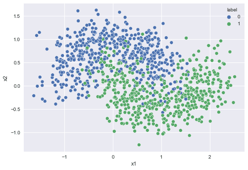

Hard voting ensemble model:

# a hard voting example
from sklearn.ensemble import VotingClassifier
from sklearn.tree import DecisionTreeClassifier
from sklearn.linear_model import LogisticRegression
from sklearn.svm import SVC

# three classifiers decision tree, logistic regression, and svm
tree_clf = DecisionTreeClassifier()
log_reg_clf = LogisticRegression()
svm_clf = SVC()

# hard voting ensemble model
voting_clf = VotingClassifier(
    estimators = [
        ('dt', tree_clf),
        ('logit', log_reg_clf),
        ('svm', svm_clf),
    ],
    voting = 'hard'  # voting type
)

# train and test each model using a loop
from sklearn.metrics import accuracy_score

for clf in (tree_clf, log_reg_clf, svm_clf, voting_clf):
    clf.fit(X_train, y_train)
    y_pred = clf.predict(X_test)
    print(clf.__class__.__name__, accuracy_score(y_test, y_pred))

Soft voting ensemble:

# a soft voting example
from sklearn.ensemble import VotingClassifier
from sklearn.tree import DecisionTreeClassifier
from sklearn.linear_model import LogisticRegression
from sklearn.svm import SVC

# three classifiers decision tree, logistic regression, and svm
tree_clf = DecisionTreeClassifier()
log_reg_clf = LogisticRegression()
svm_clf = SVC(probability=True) # probability=True to make SVC estimate class probability via CV

# soft voting ensemble model
voting_clf = VotingClassifier(
    estimators = [
        ('dt', tree_clf),
        ('logit', log_reg_clf),
        ('svm', svm_clf),
    ],
    voting = 'soft'  # voting type
)

# train and test each model using a loop
from sklearn.metrics import accuracy_score

for clf in (tree_clf, log_reg_clf, svm_clf, voting_clf):
    clf.fit(X_train, y_train)
    y_pred = clf.predict(X_test)
    print(clf.__class__.__name__, accuracy_score(y_test, y_pred))

Note that both voting ensemble models do not perform better than the best individual one but it does reduce bias by trying more models.

Bagging (Bootstrap Aggregating)

Bagging use the same model (e.g., decision tree) but train it using different random (this is why it is called random forest) subsets of the training set.

Once the predictions are made by each classifiers trained using different random subsets of the data, the result is aggregated using hard/soft voting for classification and average for regression.

Two types of subset sampling:

bagging: sampling with replacement, aka, bootstrapping (allowing the same instance to be selected more than once in one subset)
pasting: sampling without replacement

Out-of-bag Evaluation

By bootstrapping, some instances may be repeated in each subset.

If there are total m training instances, then the probability of not picking a row in a random draw is $\frac{m-1}{m}$ .

Assume each bootstrap sample contains the same number of samples as the training set and there are m bags, then the probability of an instance not picked in any bag is: ${(\frac{m-1}{m})}^m$

When m is a large number: $\displaystyle{\lim_{m \to \infty}{(\frac{m-1}{m})}^m}=e^{-1} = 0.368$

In other words, each individual model has never seen about 37% of the training data, which is called out-of-bag (OOB) instances. OOB instances can be used to validate each model without the needs to creating separate validation set.

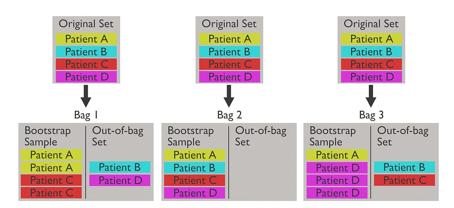
Image Source: https://en.wikipedia.org/wiki/Out-of-bag_error

Random Forest

Random Forrest is a type of Bagging Classifiers using Decision Trees. For example, if you have 1000 data points, each tree in the forest is trained using 1000 bootstrapped samples (some samples will be the same), each “bag” corresponds to a tree (an estimator).

Check the meaning of the parameters:

# random forest
from sklearn.ensemble import RandomForestClassifier

# n_estimators (default 100): The number of trees in the forest
# bootstrap (default True):Whether bootstrap samples are used when building trees. If False, the whole dataset is used to build each tree.
# oob_score: Whether to use out-of-bag samples to estimate the generalization score. Only available if bootstrap=True.
# you can specify decision tree parameters such as criterion and max_depth
rf_clf = RandomForestClassifier(n_estimators=200, bootstrap=True, oob_score=True, criterion='entropy', max_depth=5)

rf_clf.fit(X_train, y_train)
print("oob accuracy", rf_clf.oob_score_)

y_pred = rf_clf.predict(X_test)
print("random forest testing accuracy", accuracy_score(y_test, y_pred))

Boosting

Boosting refers to any Ensemble Learning method that can combine several weak predictors into a strong one.

The general idea of boosting is to train predictors sequentially, each trying to correct its predecessor.

AdaBoost

AdaBoost (Adaptive Boosting) is adaptive in the sense that subsequent weak learners are tweaked in favor of those instances misclassified by previous classifiers.

Key idea: each training instance has a weight and each weak learner has a weight, which are updated for each iteration (training each subsequent weak leaner)

The algorithm is designed as follows:

Assume there are $m$ training instances and the predictions are -1 or 1 (instead of 0 or 1):

Initialize training instance weights uniformly as $w_i^1 = \frac{1}{m}$ .
For each iteration $t$ (train one weak learner):

fit the weak learner $h_t(x)$ with the training data
calculate weighted error rate $\epsilon$ based on the follow equation (the sum of the weights of the mis-classified instances divided by the sum of all instance weights):
$\large \epsilon_t = \frac{\sum_{i=1}^m \mathbf{1}[h_t(x_i) \neq y_i] \, w_i^{(t)}}{\sum_{i=1}^mw_i^{(t)}}$
$\epsilon_t$ is 1 when predictions are all wrong.
set a weight for our weak learner based on its accuracy (eta is the learning rate):
$\alpha_t = \eta \ln \Big( \frac{1-\epsilon_t}{\epsilon_t}\Big)$
increase weights of misclassified observations: $\large w_i^{(t+1)} = w_i^{(t)} e^{-\alpha_t y_i h_t(x_i)}$ .
Renormalize weights, so that $\sum_{i=1}^m w_i^{(t+1)}=1$ .

To make predictions, AdaBoost compute the predictions of all predictors and weights them using $\alpha$ . The final prediction is the one with the majority of the weighted votes.:

H(x) = \text{sign} \Big( \sum_{t=1}^T \alpha_t h_t(x) \Big)

AdaBoost has accuracy of 0.94:

# Ada Boosting Classification
from sklearn.ensemble import AdaBoostClassifier

ada_clf = AdaBoostClassifier(n_estimators=200, algorithm="SAMME", learning_rate=0.5)
ada_clf.fit(X_train, y_train)
y_pred = ada_clf.predict(X_test)
print("AdaBoostClassifier", accuracy_score(y_test, y_pred))

Gradient Boosting

Gradient Boosting is similar to Adaboost but instead of adjusting the instance weights for each predictor, it fits the new predictor to the residual errors made by the previous predictor.

Gradient Boosting has accuracy of 0.91

# Gradient Boosting Classification
from sklearn.ensemble import GradientBoostingClassifier
gb_clf = GradientBoostingClassifier(n_estimators=200, learning_rate=0.5)
gb_clf.fit(X_train, y_train)
y_pred = gb_clf.predict(X_test)
print("GradientBoostClassifier", accuracy_score(y_test, y_pred))

XGBoost

An optimized implementation of Gradient Boosting is called Extreme Gradient Boosting (XGBoost), which is extremely fast, scalable, and portable. XGBoost is a separate package, which you can install using uv add xgboost then, you can use it as follows, which has accuracy of 0.93.

# XGBoost Classifier
import xgboost as xgb

xgb_clf = xgb.XGBClassifier()
xgb_clf.fit(X_train, y_train)
y_pred = xgb_clf.predict(X_test)
print("XGBoost Classifier accuracy:", accuracy_score(y_test, y_pred))

On this page