Linear Regression

https://www.kaggle.com/datasets/harrywang/housing

housing.csv.zip

In this lecture, we learn linear regression model.

Classification vs. Regression

• Classification: the target value is discrete/categorical, e.g, we try to predict the class label for a given data point, such as Survived/Died, Churn/Loyal.
• Regression: the target value is continuous, e.g., we aim to predict a value for the target variable, such as house price and sales.

Functional Relation vs. Statistical Relation

• For functional relations, variables can be expressed by a mathematical formula $Y = f(X)$, such as a linear relationship between the gross sales of a product (s) and its quantity sold (q) assume the fixed price is $10: sales = 10 * quantity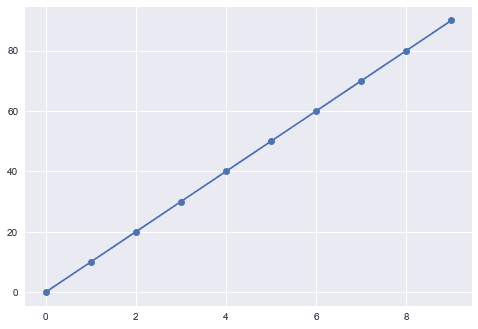

  

• For statistical relations, the data points (observations) of does not fall directly on the curve of the relationship, such as income and housing price.

  

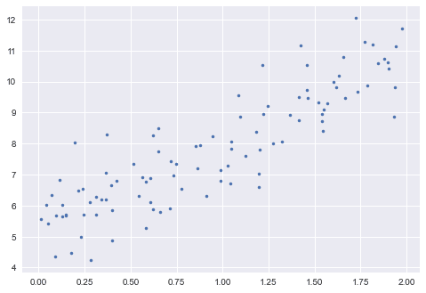
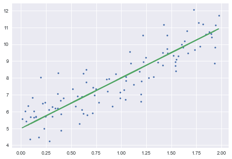
The goal of machine learning is to learn (estimate) the functional relationships from the statistical relationships to make prediction:

Linear Regression Definition

Linear regression is one of the simplest machine learning algorithms that aims to learn the linear relationship between the features and target.

A linear regression model can be informally defined as follows:

$Target = \theta_0 + \theta_1 Feature_1 + \theta_2 Feature_2 + \cdots + \theta_n Feature_n$

• Target is also called the dependent variable
• Features are also called the independent variables
• $\theta_j$ is the model parameter including:
  • the feature weights $\theta_1, \theta_2, \ldots, \theta_n$
  • the bias term (also called intercept term) $\theta_0$, this variable captures all other factors which influence the dependent/target variable other than the features.

Univariate and Multivariate Regression

A linear regression model assumes that the relationship between the target variable and the features is linear.

• Univariate: one feature. When there is only one feature (independent variable), it's called Univariate Linear Regression, such as y = 5x + 3, which is a line as shown in the example above.
• Multivariate: multiple features. When there are two or more features (independent variables), it's called Multivariate Linear Regression.
  • when there are two features, such as $y = 3x_1 + 5x_2 + 4$, it is a plane in 3D space
  • when there are three or more, such as $y = 3x_1 + 5x_2 + 7x_3 + 9$, it is a hyperplane in higher dimensional space (hard to visualize)

We use the California Housing dataset we used before - here we are going to predict the median housing price :

import numpy as np
import matplotlib.pyplot as plt
import pandas as pd
plt.style.use('ggplot')# linear regression for housing dataset

df = pd.read_csv("housing.csv")

# for simplicity let's only choose population, median_income, housing_median_age to train the model 
df = df[['population', 'median_income','housing_median_age', 'median_house_value']]

df.head()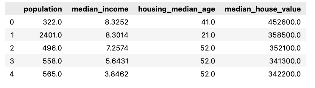

Then, the linear regression model is simply:

$MedianHouseValue = \theta_0 + \theta_1 * Population + \theta_2 * MedianIncome + \theta_3 * HousingMedianAge$

Our goal is to find the best values for $\theta_0, \theta_1, \theta_2, \ldots, \theta_n$ via training:

• first row of training data: $452600 = \theta_0 + \theta_1 * 322 + \theta_2 * 8.3252 + \theta_3 * 41.0$
• second row of training data: $358500 = \theta_0 + \theta_1 * 2401 + \theta_2 * 8.3014 + \theta_3 * 21.0$
• ...

Vector Notation

To facilitate definitions, we need to learn some vector notion for machine learning:

Vector Notation

Evaluation Metric for Linear Regression

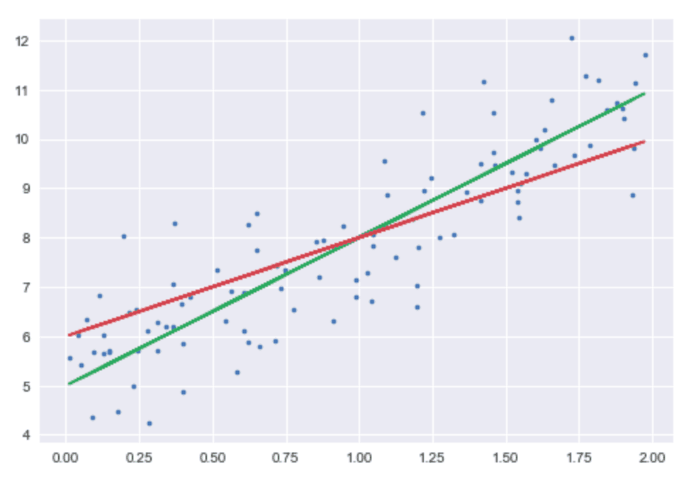
Recall that in linear regression we try to learn/estimate a linear relationship. For example, given the following two linear relationships, how do we decide which one is better?

We need to define prediction error as follows (source: https://bit.ly/3xnczu8):

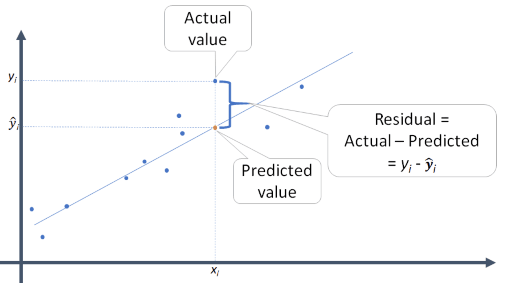
The ground truth for the $i^{th}$ instance is $y^{(i)}$

The prediction is: $\hat y^{(i)} = \mathbf{\theta}^\top \mathbf{x}^{(i)}$

The prediction error or residual is then: $\hat y^{(i)} - y^{(i)}$

For m instances, we can add up all errors in a certain way to get one of the most commonly used evaluation metrics of a regression model Root Mean Square Error (RMSE):

Our goal is to minimize RMSE.

NOTE: the RMSE is measured on the same scale with the same units as y.

In practice, it is often simpler to minimize MSE instead:

Now, we know the goal - how can we find the optimal relationship that can minimize RMSE/MSE?

• The normal equation way
• The gradient descent way (future lectures)

The Normal Equation

There exists a "closed-form" solution to find the optimal values of $\mathbf{\theta}$ that minimize MSE, which is called the Normal Equation (if you are interested in the details on deriving the normal equation using matrix calculus, check out this article: https://ayearofai.com/rohan-3-deriving-the-normal-equation-using-matrix-calculus-1a1b16f65dda)

Normal Equation is defined as (inverse matrix, transpose, ):

$\hat{\mathbf{\theta}}$ is the value of $\mathbf{\theta}$ that minimizes the cost function, i.e., MSE

# Fit linear regression using normal equation
# the ideal model apparently is y = 5 + 3x

import numpy as np
import matplotlib.pyplot as plt
plt.style.use('seaborn')

np.random.seed(42) # fix the random seed so that each run generates the same set of random numbers
X = 2 * np.random.rand(100, 1)  # generate 100 random numbers between 0 and 2 with shape (100, 1)
y = 5 + 3 * X + np.random.randn(100, 1)  # generate 100 random numbers from a normal distribution

X_with_bias = np.c_[np.ones((100,)), X] # add bias term coefficient x0 = 1 for each instance
print(X_with_bias[:2])
print('*'*50)

# we use np.linalg.inv() to calculate the inverse matrix and np.dot for matrix multiplication
# So our best model is: y = 5.215 + 2.77 * x
theta_best = np.linalg.inv(X_with_bias.T.dot(X_with_bias)).dot(X_with_bias.T).dot(y)
print(theta_best)
print('*'*50)

# given a new sets of X_new, we can predict y_pred using X dot product theta

X_new = np.array([[0.6], [0.9], [1.3]])
X_new_with_bias = np.c_[np.ones((3,1)), X_new] # add bias term coefficient x0 = 1 for each instance
y_pred = X_new_with_bias.dot(theta_best)
print(y_pred)
print('*'*50)

Output:
[[1.         0.74908024]
 [1.         1.90142861]]
**************************************************
[[5.21509616]
 [2.77011339]]
**************************************************
[[6.87716419]
 [7.70819821]
 [8.81624356]]
**************************************************

For the above example, we can use sklearn to get the same result:

# Use sklearn to do linear regression
# Singular Value Decomposition (SVD) is used to calculate the optimal solution
from sklearn.linear_model import LinearRegression
lin_reg = LinearRegression()
lin_reg.fit(X, y) # use the normal equation to train the model

print(lin_reg.predict(X_new))
print('*'*50)

print(lin_reg.intercept_, lin_reg.coef_) # exactly the same as our calculation above!

Output:
[[6.87716419]
 [7.70819821]
 [8.81624356]]
**************************************************
[5.21509616] [[2.77011339]]

Now, we can use sklearn to run linear regression for the housing dataset:

# linear regression for housing dataset
import numpy as np
import matplotlib.pyplot as plt
import pandas as pd
plt.style.use('ggplot')

df = pd.read_csv("housing.csv")

# for simplicity let's only choose population, median_income, housing_median_age to train the model 
df = df[['population', 'median_income','housing_median_age', 'median_house_value']]

# for simplicity let's only choose population, median_income, housing_median_age to train the model 
X_housing = df[['population', 'median_income','housing_median_age']]
y_housing = df['median_house_value']

# split train and test sets
from sklearn.model_selection import train_test_split
X_train_housing, X_test_housing, y_train_housing, y_test_housing = train_test_split(X_housing, y_housing, test_size=0.2, random_state=42)

# setup the linear regression model
from sklearn.linear_model import LinearRegression
lin_reg_housing = LinearRegression()
lin_reg_housing.fit(X_train_housing, y_train_housing)

# the fitted model is
# median_house_value = -17768 + 2.975 * population + 43399 * median_income + 1828 * housing_median_age
# 1.82807894e+03 is the scientific notation: https://www.mathsisfun.com/numbers/scientific-notation.html
print(f'The intercept is {lin_reg_housing.intercept_} and coefficient is {lin_reg_housing.coef_}')

y_pred_housing = lin_reg_housing.predict(X_test_housing)

# calculate MSE and RMSE
# NOTE: the RMSE is measured on the same scale with the same units as y.
# RMSE is sort of the "average prediction error"

from sklearn.metrics import mean_squared_error
lin_mse_housing = mean_squared_error(y_test_housing, y_pred_housing) 
lin_rmse_housing = np.sqrt(lin_mse_housing)

print(f'Median house value mean is {df.median_house_value.mean():.3f}, std is: {df.median_house_value.std():.3f}')
print(f'The RMSE is {lin_rmse_housing:.3f}, which is ~{lin_rmse_housing/df.median_house_value.std():.2f} std')

# train the final model using ALL data
# the intercept and coefficients are slightly different from the training data result
lin_reg_housing.fit(X_housing, y_housing)
print(f'The intercept is {lin_reg_housing.intercept_} and coefficient is {lin_reg_housing.coef_}')

Questions:

• Do you still need Grid Search to tune linear regression model? why?
• Do you still need to build a pipeline to do the necessary pre-processing?

Vector Notation