Data Preprocessing

housing-dirty.csv.zip

We will cover the followings:

• Missing Data
• Outlier
• Standardization
• Categorical data encoding

We will two datasets:

df_country = pd.read_csv('countries-2021.csv')
df_housing = pd.read_csv('housing-dirty.csv')

How to drop rows or columns

# use country dataset
df_country.drop([1, 3, 4])  # delete row with index 1, 3, 4 default axis=0
df_country.drop(['gdp', 'area'], axis=1)  # delete 'gdp' and 'area' columns
df_country.drop(['population'], axis=1, inplace=True)  # delete 'gdp' and 'area' columns

Missing Data

Find missing data:

df_housing.isnull().sum()  # total count
df_housing.isnull().sum()/len(df)  # ratio

longitude             0.000000
latitude              0.000000
housing_median_age    0.111095
total_rooms           0.000000
total_bedrooms        0.875436
population            0.000000
households            0.000000
median_income         0.000145
median_house_value    0.000000
ocean_proximity       0.101938

Handling missing data:

There are basically three ways we can handle the missing data. The key is to understand when to use which method and the potential consequences.

1. delete columns with missing data (when most of the values in the column are missing and the feature is not that critical). Given that 88% of total_bedrooms is missing, we can drop that column.

df_housing.drop('total_bedrooms', axis=1, inplace=True)

1. delete rows with missing data (when the number of rows with missing data are not large)

   • delete all rows with missing data in any column df.dropna() - given that the missing data in housing_median_age and ocean_proximity is about 10% of total data - we cannot afford to delete them all.
   • delete rows with missing data in specific columns. Given only 3 rows are missing for median_income, we can drop those three rows:

   df_housing.dropna(subset=['median_income'])

2. impute the missing values with different imputation strategy (NOTE: imputed values may not be the real values)

   .fillna() can be used to fill the missing values。

   • mean: replace missing values using the mean along each column. Can only be used with numeric data

   df_housing.housing_median_age.fillna(df.housing_median_age.mean(), inplace=True)

   • median: replace missing values using the median along each column. Can only be used with numeric data
   • most_frequent: replace missing using the most frequent value along each column. Can be used with strings or numeric data. If there is more than one such value, only the smallest is returned.

   # .idxmax()/.idxmin() returns the index of first occurrence of max/min over requested axis
   most_freq = df_housing.ocean_proximity.value_counts().idxmax()
   df_housing.ocean_proximity.fillna(most_freq, inplace=True)

   • constant: replace missing values with fill_value. Can be used with strings or numeric data.

   .fillna() can also use the following methods to handle both numerical and categorical missing values, such as .fillna(method='bfill') or .fillna(method='ffill'):

   • backfill/bfill: use next valid observation to fill gap
   • pad / ffill: propagate last valid observation forward to next valid

   NOTE that there are more sophisticated imputation strategies, such as using the longitude and latitude to impute the ocean proximity, which can have more accurate imputation results.

Outliers

use box plots to check the outliers visually:

df_housing.boxplot(figsize=(20, 5))  # for all numerical features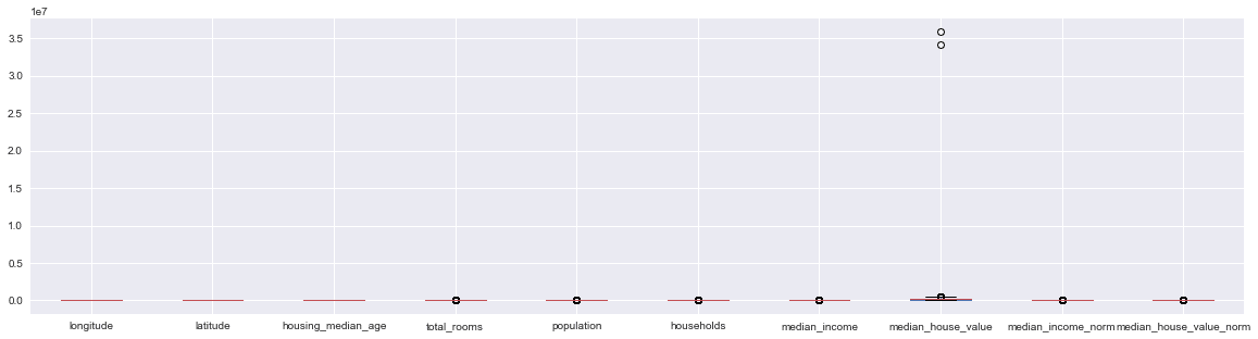

z-score:

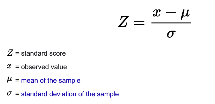
A z-score measures how far a data point is away from the mean (in terms of how many standard deviations) , e.g., z-score is 0 means the data point’s value equals to the mean.

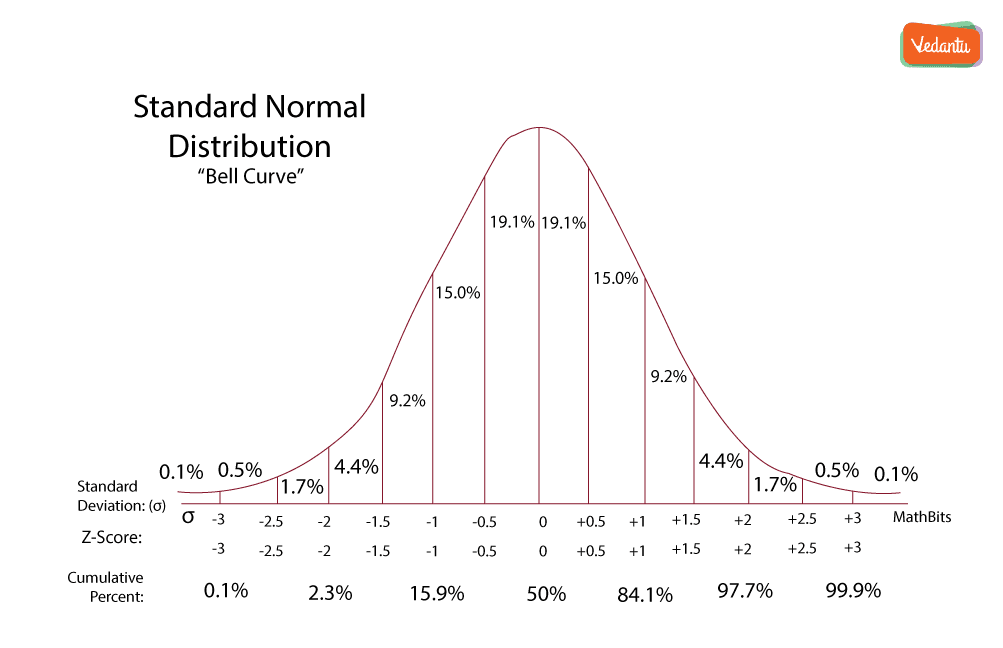
Outliers can be defined as any data point that is 3 or more standard deviations away from the mean, i.e., z-score >= 3 or z-score ≤ -3

# use scipy to get the z-score
from scipy import stats
import numpy as np
stats.zscore(df_housing.median_house_value)

or you can manually calculate the z-score:

# manual calculate z-score
(df_housing.median_house_value - df_housing.median_house_value.mean())/df_housing.median_house_value.std() 

we can then remove all rows with outliers.

Use z-scores to remove outliers:

# create a new column
df_housing['median_house_value_z'] = stats.zscore(df_housing.median_house_value)
# select rows with abs z-score between -3 and 3
df_housing = df_housing[(df_housing.median_house_value_z > -3) & (df_housing.median_house_value_z < 3)]

z-score must be updated after removing outliers

# update z-score after removing outliers
df_housing['median_house_value_z'] = stats.zscore(df_housing.median_house_value)

Now, plot again - less outliers - (still some outliers in box plot definition: outliers are identified as 1.5 IQR away from the median, which is about 2.7 $\sigma$ away from the mean, see https://towardsdatascience.com/why-1-5-in-iqr-method-of-outlier-detection-5d07fdc82097 for a detailed explanation).

df_housing.median_house_value.plot.box()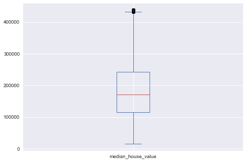

Standardization

Why standardization:

df_housing[['median_income', 'median_house_value']].plot()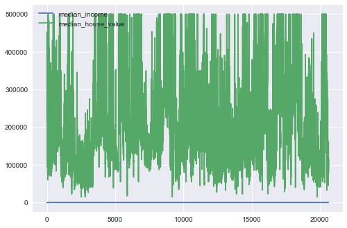

Features (columns) are often measured at different scales, e.g., 10 for house value is not same for 10 for income. Standardization brings the features to the same scale using their z-score, i.e., the features will be rescaled so that they’ll have the properties of a standard normal distribution with $\mu = 0$, $\sigma = 1$)

# standardization using z-score
df_housing['median_income_z'] = stats.zscore(df_housing.median_income)
df_housing['median_house_value_z'] = stats.zscore(df_housing.median_house_value)

now plot the standardized features - they are on the same scale:

df_housing[['median_income_z', 'median_house_value_z']].plot()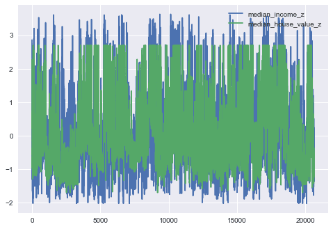

Categorical Data Encoding

Machine learning models require all variables to be numeric, which means the categorical data must be encoded to numbers before it can be used to fit and evaluate models.

Two most popular techniques are:

• Ordinal Encoding
• One-Hot Encoding

Ordinal Encoding

In ordinal encoding, each unique category value is assigned an integer value, such as 'North America' is 0, 'Asia' is 1, 'Europe' is 2, and 'South America' is 3.

# create a dict mapper then use .replace() to encode
ordinal_mapper = {'North America': 0, 'Asia': 1, 'Europe': 2, 'South America': 3}
df_country['continent_encoded'] = df_country.continent.replace(ordinal_mapper)
df_country[['continent', 'continent_encoded']]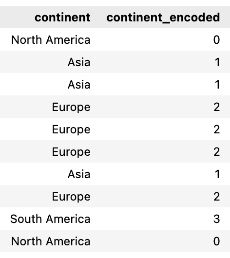

You can use the following line to get the ordinal mapper:

ordinal_mapper = dict(zip(df_country.continent.unique(), np.arange(df_country.continent.nunique())))

The integer encoding above implies an ordinal relationship, such as 'South America': 3 is “after” or “greater than” 'Asia': 1, which may be misleading to the model and result in poor performance or unexpected results.

One-Hot Encoding

In one-hot encoding, one new binary variable is added for each unique category value in the variable:

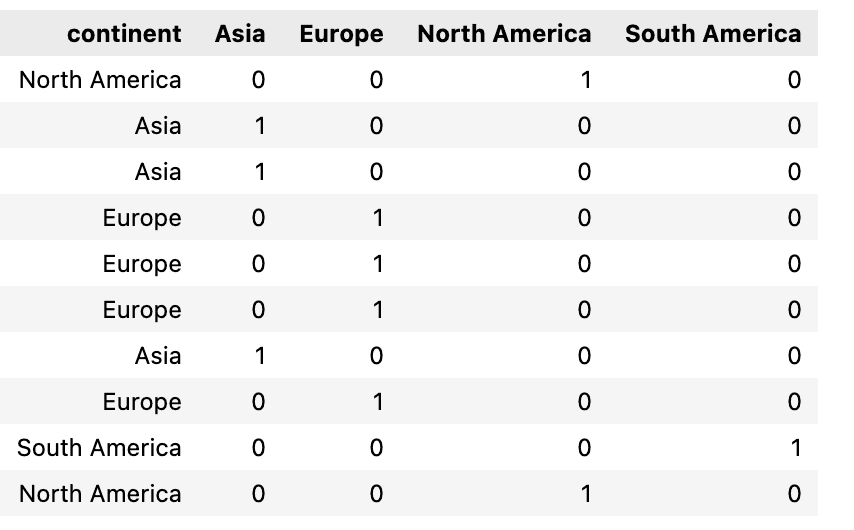
df_dummy = pd.get_dummies(df_country.continent)  # returns a data frame
pd.concat([df_country, df_dummy], axis=1)  # concatenate the data frame

For categorical features with large unique values, one-hot encoding will create a large number of new features that can make the model very complex.

• use domain knowledge to combine the categories to a smaller number and then apply one-hot encoding, such as mapping 50 states to 5 regions (Northeast, Southwest, West, Southeast, and Midwest) and then do the one-hot encoding.
• use dimensionality reduction techniques such as principal component analysis (PCA)

scikit-learn Package

As we will see later in this semester, scikit-learn package provides easier ways to do missing data imputation, standardization, ordinal encoding, and one-hot encoding.