
Baseline Model-based Prediction
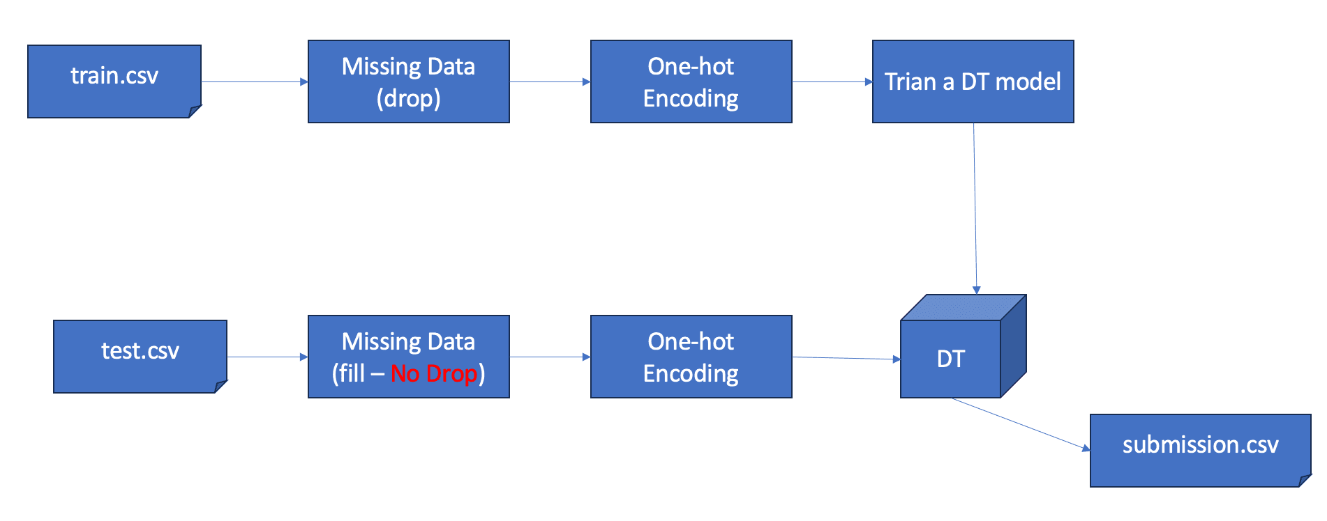
We create a basic Decision Tree model with all default settings to show the key steps for building a baseline model-based prediction (no model selection, no model tuning, etc. which will be covered later).
The key steps are:
- select features and target
- data pre-processing
- handle missing data
- handle outliers
- standardization
- categorical data encoding
- build a machine learning model
- use the model to predict (NOTE: the testing data must go through the same data pre-processing steps to match the training data format)
# read training data
df_train = pd.read_csv('train.csv')

# specify features and target (remove unuseful features)
df_train = df_train[['Survived', 'Sex', 'Pclass', 'SibSp', 'Fare', 'Embarked']]

# data preprocessing
df_train.dropna(inplace=True)  # drop missing values

gender_dummies = pd.get_dummies(df_train.Sex)  # one-hot encoding for Sex
embarked_dummies = pd.get_dummies(df_train.Embarked)  # one-hot encoding for Embarked

df_num = df_train[['Survived', 'Pclass', 'SibSp', 'Fare']]  # choose numerical features

df_train_processed = pd.concat([df_num, gender_dummies, embarked_dummies], axis=1)  # concatenate all dataframes into one
df_train_processed.head()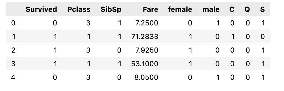
# get features and target
X = df_train_processed.drop('Survived', axis=1)
y = df_train_processed['Survived']
# train a DT model by using all default settings
# note the default criterion='gini', which can be changed to criterion='entropy'
from sklearn.tree import DecisionTreeClassifier
tree_clf = DecisionTreeClassifier()
tree_clf.fit(X, y)prepare test samples (two passengers):
# passenger 1 who bought a class 3 ticket at $8.5 with no siblings / spouses, Jack ?
# passenger 2 who bought a first class ticket at $88 with no siblings / spouses, Rose ?

p = {
    'Pclass': [3, 1], # [] needed, even for one row
    'SibSp': [0, 0],
    'Fare': [7, 85],
    'female': [0, 1],
    'male': [1, 0],
    'C': [0, 0],
    'Q': [0, 0],
    'S': [1, 1],
}

df_p = pd.DataFrame(p)
df_p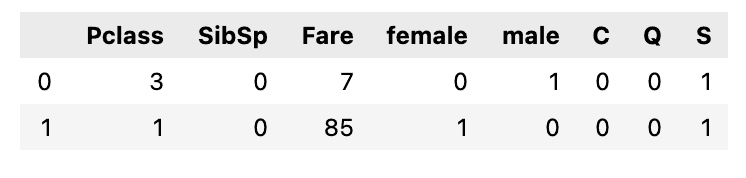
# make predictions
p_pred = tree_clf.predict(df_p)
p_pred

array([0, 1])  # this means first passenger predicted dead, second one survived
Get test dataset from Kaggle.
# this is training dataframe, the testing dataframe must match this format
X.head()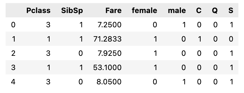
df_test = pd.read_csv('test.csv')

# process test dataset for prediction
# NOTE: we CANNOT remove any rows from the test data for Kaggle prediction scoring

# read testing data
df_test = pd.read_csv('test.csv')

# select the same features as in training data X + PassengerId which we will need for submission
df_test = df_test[['PassengerId', 'Sex', 'Pclass', 'SibSp', 'Fare', 'Embarked']].copy()

# check missing values
df_test.isnull().sum()

PassengerId    0
Sex            0
Pclass         0
SibSp          0
Fare           1
Embarked       0
dtype: int64
We cannot remove rows for Kaggle testing dataset, so we use mean to fill the missing data:
# we have to impute the missing values for Kaggle prediction scoring
# we just fill the missing fare with the mean
fare_mean = df_test.Fare.mean()
df_test.Fare.fillna(fare_mean, inplace=True)

# sanity check for missing values
df_test.isnull().sum()

PassengerId    0
Sex            0
Pclass         0
SibSp          0
Fare           0
Embarked       0
dtype: int64
# test data encoding
gender_dummies_test = pd.get_dummies(df_test.Sex) # one-hot encoding for Sex
embarked_dummies_test = pd.get_dummies(df_test.Embarked) # one-hot encoding for Embarked
df_num_test = df_test[['Pclass', 'SibSp', 'Fare']] # choose numerical features
X_test = pd.concat([df_num_test, gender_dummies_test, embarked_dummies_test], axis=1) # concatenate all dataframes into one
X_test.head() # this should match the training X format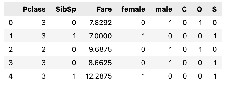
Make predictions:
y_hat = tree_clf.predict(X_test)
y_hat  # a numpy array with prediction results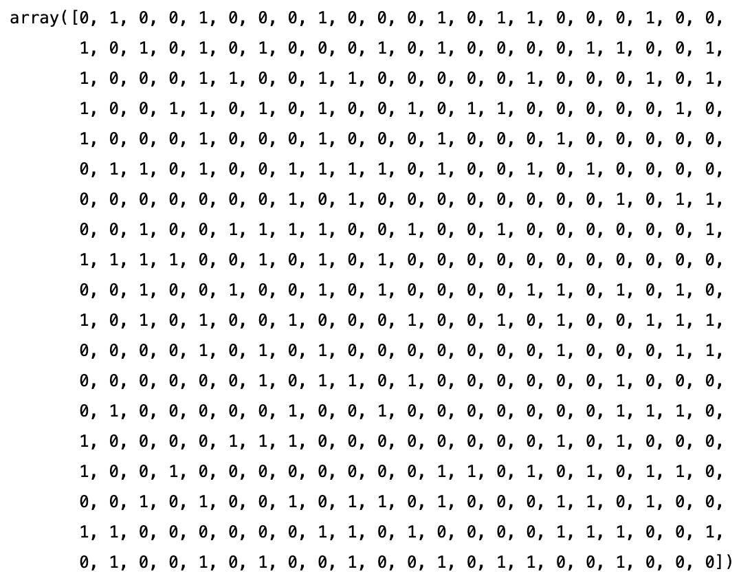
# combine the final dataframe from two arrays
df_submit_dt = pd.DataFrame({
                              'PassengerId': df_test.PassengerId,
                              'Survived': y_hat,
                            })
df_submit_dt.head()

# export the csv for submission
df_submit_dt.to_csv('submit_simple_dt.csv', index=False)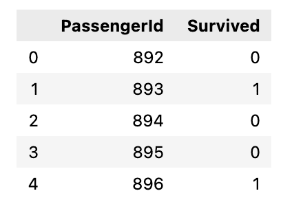
This basic model-based prediction gets 0.7799 accuracy, which beats the gender-based prediction baseline.

Next, we will learn how models are evaluated and how to do model evaluation when we only have training data (no need to submit to Kaggle)
Tree Visualization (Optional)
You can visualize the decision tree as follows:
from sklearn import tree
fig, ax = plt.subplots(figsize=(25, 20))
tree.plot_tree(tree_clf)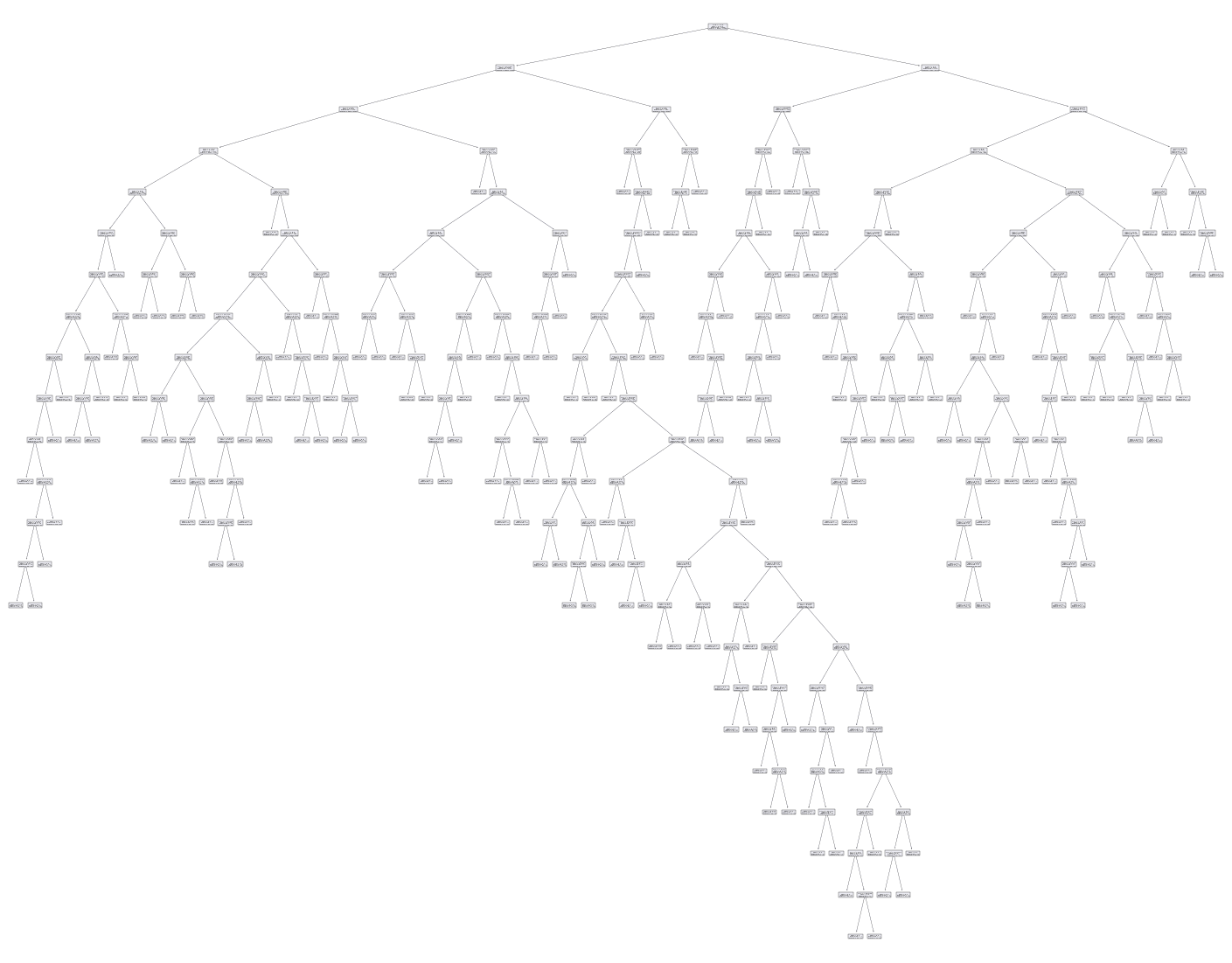
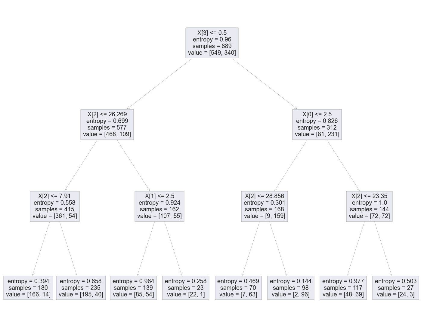
The decision tree above this very complicated which may indicate overfitting (will be introduced later). We can tune the model by creating a new model with different parameters:
# a tree using entropy and max-depth 3
tree_clf_simple = DecisionTreeClassifier(criterion='entropy', max_depth=3)
tree_clf_simple.fit(X, y)  # a new model is trained using the same data

# show the tree
fig, ax = plt.subplots(figsize=(25, 20))
tree.plot_tree(tree_clf_simple)
Note the tree has not feature names and labels - hard to interpret:
# get feature and class names for visualization
cls_names = ['died', 'survived']  # died 0, survived 1
cls_names

feature_list = X.columns.values
feature_list

array(['Pclass', 'SibSp', 'Fare', 'female', 'male', 'C', 'Q', 'S'], dtype=object)
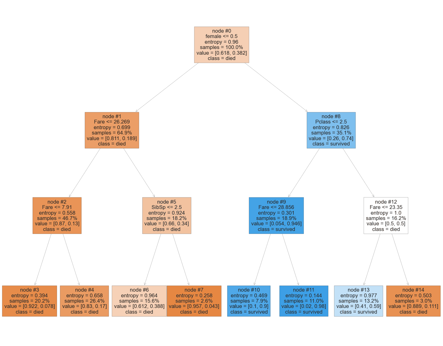
show the tree again with new settings:
fig, ax = plt.subplots(figsize=(25, 20))
tree.plot_tree(
    tree_clf,
    feature_names=feature_list,
    class_names=cls_names,
    filled=True,
    proportion=True,
    node_ids=True
    )
Yes to the left, No to the right - let’s make some predictions and see how this tree works.
df_p # test data with two passengers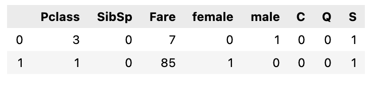
# use the new tree to make predictions

p_pred_simple = tree_clf_simple.predict(df_p)
p_pred_simple

array([0, 1])
We can walk through the tree to see how the predictions were made using the tree.